How to plot metabolite concentrations in R?

The data source

Let’s say we have the final concentrations of following metabolites from three strains of bacteria:

Glucose
Ethanol
Succinate
Acetate
Formate
Lactate

Each strain was grown in triplicates, so we have three values of each metabolite for each strain.

Load `tidyverse`

We will first load the tidyverse library which contains all the functions that we are going to need here.

library(tidyverse)

Read data

The data for this example is stored in an excel file which would read first.

data <- readxl::read_excel('data/fermentation_products.xlsx')
data

## # A tibble: 18 × 4
##    Product   Strain_A Strain_B Strain_C
##    <chr>        <dbl>    <dbl>    <dbl>
##  1 Glucose       1.59     1.73     1.72
##  2 Glucose       1.65     1.82     1.68
##  3 Glucose       1.45     1.86     1.74
##  4 Succinate     0.08     0.07     1.2 
##  5 Succinate     0.1      0.05     1.23
##  6 Succinate     0.11     0.08     1.3 
##  7 Lactate       0.26     0.12     0.15
##  8 Lactate       0.28     0.1      0.14
##  9 Lactate       0.32     0.09     0.18
## 10 Formate       1.29     1.65     2.72
## 11 Formate       1.34     1.74     2.71
## 12 Formate       1.38     1.87     2.6 
## 13 Acetate      10.5     14.3      8.73
## 14 Acetate      10.7     15.6      9.47
## 15 Acetate       9.4     16.3      6.52
## 16 Ethanol      15.7     21.2     30.3 
## 17 Ethanol      14.3     19.0     32.2 
## 18 Ethanol      13.6     22.8     33.8

The data as seen above, has four columns. First column, “Product”, represents the product, each of the other columns represents measured concentration of the metabolite in grams per litre. Each metabolite will occur three times in the ‘Product’ column as there are three replicates.

Rearrange data

We will rearrange our data so as not to have separate columns for each strain. We will rearrange it such that we have three columns, Product, Strain and Amount.

This is called as pivoting which is done by pivot_longer function. The resulting data will have nine instances of each metabolite in the ‘Product’ column.

data %>%
  pivot_longer(!Product,
               names_to='Strain',
               values_to='Amount')

## # A tibble: 54 × 3
##    Product   Strain   Amount
##    <chr>     <chr>     <dbl>
##  1 Glucose   Strain_A   1.59
##  2 Glucose   Strain_B   1.73
##  3 Glucose   Strain_C   1.72
##  4 Glucose   Strain_A   1.65
##  5 Glucose   Strain_B   1.82
##  6 Glucose   Strain_C   1.68
##  7 Glucose   Strain_A   1.45
##  8 Glucose   Strain_B   1.86
##  9 Glucose   Strain_C   1.74
## 10 Succinate Strain_A   0.08
## # ℹ 44 more rows

Plot

The rearranged data can now be easily plotted as a bar graph. Here is how we combine the rearrangement and plotting statements in one piped code.

data %>%
  pivot_longer(!Product,
               names_to='Strain',
               values_to='Amount') %>%
  ggplot(mapping = aes(x=Product,
                       y = Amount,
                       fill=Strain)) +
  geom_bar(stat="identity",
           position = 'dodge')+
  theme_bw()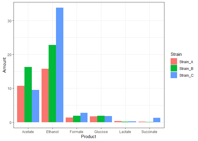

The above plot may look all right, but it doesn’t represent our data. The three replicates are plotted above one another.

In the data such as ours, we will plot the mean of the three replicates and the standard deviations in the measurements as the error bars. So, first nee to calculate the means and standard deviations in our data.

Let’s start again by reading the data.

data <- readxl::read_excel('data/fermentation_products.xlsx')
data

## # A tibble: 18 × 4
##    Product   Strain_A Strain_B Strain_C
##    <chr>        <dbl>    <dbl>    <dbl>
##  1 Glucose       1.59     1.73     1.72
##  2 Glucose       1.65     1.82     1.68
##  3 Glucose       1.45     1.86     1.74
##  4 Succinate     0.08     0.07     1.2 
##  5 Succinate     0.1      0.05     1.23
##  6 Succinate     0.11     0.08     1.3 
##  7 Lactate       0.26     0.12     0.15
##  8 Lactate       0.28     0.1      0.14
##  9 Lactate       0.32     0.09     0.18
## 10 Formate       1.29     1.65     2.72
## 11 Formate       1.34     1.74     2.71
## 12 Formate       1.38     1.87     2.6 
## 13 Acetate      10.5     14.3      8.73
## 14 Acetate      10.7     15.6      9.47
## 15 Acetate       9.4     16.3      6.52
## 16 Ethanol      15.7     21.2     30.3 
## 17 Ethanol      14.3     19.0     32.2 
## 18 Ethanol      13.6     22.8     33.8

Get mean values

We will use two functions, group_by and summarize to get the mean values of the replicate experiments.

n_data <- data %>%
  group_by(Product) %>%
  summarize(A = mean(Strain_A),
            B = mean(Strain_B),
            C = mean(Strain_C),
            )
n_data

## # A tibble: 6 × 4
##   Product         A       B      C
##   <chr>       <dbl>   <dbl>  <dbl>
## 1 Acetate   10.2    15.4     8.24 
## 2 Ethanol   14.5    21.0    32.1  
## 3 Formate    1.34    1.75    2.68 
## 4 Glucose    1.56    1.80    1.71 
## 5 Lactate    0.287   0.103   0.157
## 6 Succinate  0.0967  0.0667  1.24

In the above table, we see that we now have only one instance of each metabolite and each value represents the mean value of the metabolite in a particular strain.

We also assigned the column names so that it contain only the name of the trains.

This data is now suitable to do pivot_longer as seen before.

n_data_long <- n_data %>%
  pivot_longer(!Product,
               names_to = 'Strain',
               values_to = 'mean')
  
n_data_long

## # A tibble: 18 × 3
##    Product   Strain    mean
##    <chr>     <chr>    <dbl>
##  1 Acetate   A      10.2   
##  2 Acetate   B      15.4   
##  3 Acetate   C       8.24  
##  4 Ethanol   A      14.5   
##  5 Ethanol   B      21.0   
##  6 Ethanol   C      32.1   
##  7 Formate   A       1.34  
##  8 Formate   B       1.75  
##  9 Formate   C       2.68  
## 10 Glucose   A       1.56  
## 11 Glucose   B       1.80  
## 12 Glucose   C       1.71  
## 13 Lactate   A       0.287 
## 14 Lactate   B       0.103 
## 15 Lactate   C       0.157 
## 16 Succinate A       0.0967
## 17 Succinate B       0.0667
## 18 Succinate C       1.24

Get standard deviation

Now that we have the data of means, we will calculate the standard deviation in similar way.

First get the standard deviation values.

sds <- data %>%
  group_by(Product) %>%
  summarize(A = sd(Strain_A),
            B = sd(Strain_B),
            C = sd(Strain_C))

sds

## # A tibble: 6 × 4
##   Product        A      B      C
##   <chr>      <dbl>  <dbl>  <dbl>
## 1 Acetate   0.690  1.01   1.53  
## 2 Ethanol   1.11   1.92   1.73  
## 3 Formate   0.0451 0.111  0.0666
## 4 Glucose   0.103  0.0666 0.0306
## 5 Lactate   0.0306 0.0153 0.0208
## 6 Succinate 0.0153 0.0153 0.0513

And rearrange by pivot_longer.

sds_long <- sds %>%
  pivot_longer(!Product,
               names_to = 'Strain',
               values_to = 'stdev')

sds_long

## # A tibble: 18 × 3
##    Product   Strain  stdev
##    <chr>     <chr>   <dbl>
##  1 Acetate   A      0.690 
##  2 Acetate   B      1.01  
##  3 Acetate   C      1.53  
##  4 Ethanol   A      1.11  
##  5 Ethanol   B      1.92  
##  6 Ethanol   C      1.73  
##  7 Formate   A      0.0451
##  8 Formate   B      0.111 
##  9 Formate   C      0.0666
## 10 Glucose   A      0.103 
## 11 Glucose   B      0.0666
## 12 Glucose   C      0.0306
## 13 Lactate   A      0.0306
## 14 Lactate   B      0.0153
## 15 Lactate   C      0.0208
## 16 Succinate A      0.0153
## 17 Succinate B      0.0153
## 18 Succinate C      0.0513

Now, we will add the standard deviation values into the data table that contains the mean values.

n_data_long <- n_data_long %>%
  mutate(stdev = sds_long$stdev)

n_data_long

## # A tibble: 18 × 4
##    Product   Strain    mean  stdev
##    <chr>     <chr>    <dbl>  <dbl>
##  1 Acetate   A      10.2    0.690 
##  2 Acetate   B      15.4    1.01  
##  3 Acetate   C       8.24   1.53  
##  4 Ethanol   A      14.5    1.11  
##  5 Ethanol   B      21.0    1.92  
##  6 Ethanol   C      32.1    1.73  
##  7 Formate   A       1.34   0.0451
##  8 Formate   B       1.75   0.111 
##  9 Formate   C       2.68   0.0666
## 10 Glucose   A       1.56   0.103 
## 11 Glucose   B       1.80   0.0666
## 12 Glucose   C       1.71   0.0306
## 13 Lactate   A       0.287  0.0306
## 14 Lactate   B       0.103  0.0153
## 15 Lactate   C       0.157  0.0208
## 16 Succinate A       0.0967 0.0153
## 17 Succinate B       0.0667 0.0153
## 18 Succinate C       1.24   0.0513

Plot

Now this data is suitable for plotting. As above, we will use ggplot with its geom_bar function.

Plot means

We will first plot the means and step by step add other things to make our plot.

n_data_long %>%
  ggplot(mapping = aes(x = Product,
                       y = mean,
                       fill = Strain)) +
  geom_bar(stat='identity',
           position = 'dodge',
           width = 0.8)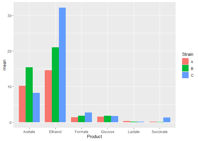

Plot means and standards deviations

To the above plot we will add the layer of error bars.

n_data_long %>%
  ggplot(mapping = aes(x=Product, y=mean, fill=Strain)) +
  geom_bar(stat='identity',
           position = 'dodge',
           width = 0.8) +
  geom_errorbar(mapping = aes(x = Product,
                              ymin = mean - stdev,
                              ymax = mean + stdev),
                width = 0.2,
                position = position_dodge(width=0.8)) +
  theme_bw()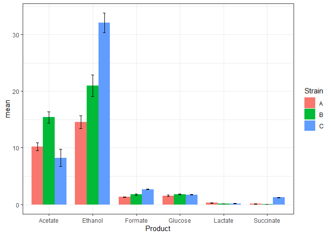

Theme

We will use the theme_bw theme.

n_data_long %>%
  ggplot(mapping = aes(x=Product, y=mean, fill=Strain)) +
  geom_bar(stat='identity',
           position = 'dodge',
           width = 0.8) +
  geom_errorbar(mapping = aes(x = Product,
                              ymin = mean - stdev,
                              ymax = mean + stdev),
                width = 0.2,
                position = position_dodge(width=0.8)) +
  theme_bw()

Add axes labels and plot title

n_data_long %>%
  ggplot(mapping = aes(x=Product, y=mean, fill=Strain)) +
  geom_bar(stat='identity',
           position = 'dodge',
           width = 0.8) +
  geom_errorbar(mapping = aes(x = Product,
                              ymin = mean - stdev,
                              ymax = mean + stdev),
                width = 0.2,
                position = position_dodge(width=0.8)) +
  theme_bw() +
  labs(title = 'Fermetation product titres',
       y = 'Concetration (g/l)')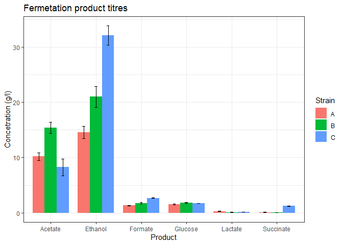

Facet wrap

The above plot looks good but some of the products are too low in concentration. We could barely view their bars. facet_wrap function can be used to separate the plot into subplots so that each product gets its own subplot.

n_data_long %>%
  ggplot(mapping = aes(x=Product, y=mean, fill=Strain)) +
  geom_bar(stat='identity',
           position = 'dodge',
           width = 0.8) +
  geom_errorbar(mapping = aes(x = Product,
                              ymin = mean - stdev,
                              ymax = mean + stdev),
                width = 0.2,
                position = position_dodge(width=0.8)) +
  theme_bw() +
  labs(title = 'Fermetation product titres',
       y = 'Concetration (g/l)') +
  facet_wrap(vars(Product), nrow=2, scales='free')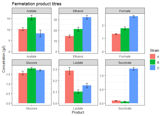

The above graph looks much better.

Combining everything into functions

When we are going to use above code for our work, it would be very inconvenient run all lines of code each time we want to make the graph. Instead, we will write function such that we can run all the above code in one line and get the plot.

We will divide the code into two function, one for data wrangling and another for data visualization. A third function would call these two function so that we can just call the third function and draw the graph.

The three functions are written below.

# data wrangling
transform_data <- function(data){
  
  # calculate means and pivot longer
  n_data_long <- data %>%
    group_by(Product) %>%
    summarize(A = mean(Strain_A),
              B = mean(Strain_B),
              C = mean(Strain_C),
    ) %>%
    pivot_longer(!Product,
                 names_to = 'Strain',
                 values_to = 'mean')
  
  # calculate st dev and pivot longer
  sds <- data %>%
    group_by(Product) %>%
    summarize(A = sd(Strain_A),
              B = sd(Strain_B),
              C = sd(Strain_C)) %>%
    pivot_longer(!Product,
                 names_to = 'Strain',
                 values_to = 'stdev')
  
  
  # add st dev column to the n_data
  n_data_long <- n_data_long %>%
    mutate(stdev = sds_long$stdev)
  
  return(n_data_long)
  }
  

# data plotting
ferm_plot <- function(data){
  
  #plot
  data %>%
    ggplot(mapping = aes(x=Product, y=mean, fill=Strain)) +
    geom_bar(stat='identity',
             position = 'dodge',
             width = 0.8) +
    geom_errorbar(mapping = aes(x = Product,
                                ymin = mean - stdev,
                                ymax = mean + stdev),
                  width = 0.2,
                  position = position_dodge(width=0.8)) +
    theme_bw() +
    labs(title = 'Fermetation product titres',
         y = 'Concetration (g/l)') +
    facet_wrap(vars(Product), nrow=2, scales='free')
  
  }


# call above two functions
plot_data <- function(data){
  n_data_long <- transform_data(data)
  ferm_plot(n_data_long)
}

Now when we have these three functions, we can plot the graph in two lines.

Read the data.
Call the plot_data function.

# utilize the above function
data <- readxl::read_excel('data/fermentation_products.xlsx')

plot_data(data)

And we get the plot.

Analytics Notes